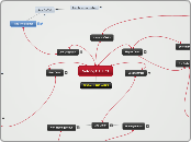
Solving O.D.E.'S

Begin by placing the equaiton in standard form.Standard Form:Ay'+P(t)y=Q(t), Where A=1.

The Integrating factor will be: e^(Integral of P(t)dt)With this method, you need not include an integration constant when calculating the integrating factor.

Multiply both sides of the DE by the integrating factor and then integrate both sides.The left side will always become:Iy, with I=Integrating Factor.Ex.y'+2y=3e^tI=e^(Integral of 2dt)=e^(2t)(e^(2t))(y'+2y)=(3e^t)(e^(2t))Multiply Through To Get:d/dt(ye^2t)=3e^3tThen Integrate Both Sides:ye^(2t)=e^(3t)+C

Higher Order DE's can be evaluated in the same manner as a second order DE. Begin by determining homogeneous or non homogeneous.

Place all the y variables on the left side of the DE and t variables on the right side of the DE.Homogenous if the Right Side of DE = 0.The general form of a Homogeneous third order DE will be:ay'''+by''+cy'+dy=0

Place all the y variables on the left side of the DE and t variables on the right side of the DE.Non-Homogenous if the Right Side of DE does not = 0.The general form of a Non-Homogeneous third order DE will be:ay'''+by''+cy'+dy=f(t)Where f(t) is known as the "Forcing Function"

One Being the Highest Power Derivative in the DE.*Note: If you are given initial conditions along with the DE, first solve the DE and then apply the initial conditions to solve for any integration constants.

Can you integrate both sides of the equation directly?Ex:dy=(x^2)dxIntegrate to Get:y=((x^3)/3)+C

Ex:dy=(x^2)dx Integrate to Get:y=((x^3)/3)+C

One Being the Highest Power Derivative in the DE.*Note: If you are given initial conditions along with the DE, first solve the DE and then apply the initial conditions to solve for any integration constants.

Place all the y variables on the left side of the DE and t variables on the right side of the DE.Homogenous if the Right Side of DE = 0.The general form of a Homogeneous second order DE will be:ay''+by'+cy=0

Ex:ay''+by'+cy=0Becomes:ar^2+br+c=0

Solve for the roots of the characteristic equation.Call them r1 & r2

r1 & r2 are real numbers and do not equal each other.

c1 and c2 are arbitrary constants. To solve for c1 and c2 initial conditions must be provided. If initial conditions are provided use them along with this solution to solve an algebraic system of equations for c1 and c2.

r1 & r2 are real numbers and are equal to each other.

c1 and c2 are arbitrary constants. To solve for c1 and c2 initial conditions must be provided.If initial conditions are provided use them along with this solution to solve an algebraic system of equations for c1 and c2.

r1 & r2 are imaginary numbers.Ex:r1=A+iBr2=A-iB

c1 and c2 are arbitrary constants. To solve for c1 and c2 initial conditions must be provided.If initial conditions are provided use them along with this solution to solve an algebraic system of equations for c1 and c2.

This method involves transforming the given DE into an equivalent system of first order DE's.Click on the globe to the right to obtain the worksheet for transfroming a higher order DE into a system of first order DE's.Then move on to solving the system in the next step.

Place all the y variables on the left side of the DE and t variables on the right side of the DE.Homogenous if the Right Side of DE = 0.The general form of a Homogeneous third order DE will be:ay'''+by''+cy'+dy=0

Ex:ay'''+by''+cy'+dy=0Becomes:ar^3+br^2+cr+d=0The same form follows for any order DE. Just form the appropriate characteristic equation.

Solve for the roots of the characteristic equation.Call them r1, r2, r3, and so on for however many roots your characteristic equation has.Then determine if you have real, repeated, or imaginary roots.Note: For a higher order DE, you will very likely have a combination of more than one type of root. Meaning real and imaginary roots for the same DE.

The general solution to this DE, will be the combination of all of the solution pieces.Example: For a DE with one real and two imaginary roots, the general solution is:y(t)=c1e^(r1t)+(e^(At)(c2cosBt+c2sinBt))

The roots are real unequal numbers.

c1, c2, and so on are arbitrary constants. To solve for them initial conditions must be provided. If initial conditions are provided use them along with this solution to solve an algebraic system of equations for and constants.

Roots are repeated real numbers.Meaning r1=r2 and so on.

c1, c2, and so on are arbitrary constants. To solve for them initial conditions must be provided.If initial conditions are provided use them along with the general solution to solve an algebraic system of equations for the constants.

r1, r2, and so on are imaginary numbers.Ex:r1=A+iBr2=A-iB

c1, c2 and so on are arbitrary constants. To solve for them initial conditions must be provided.If initial conditions are provided use them along with the general solution to solve an algebraic system of equations for the constants.

Follow these steps to solve the system of DE's. For Help with the steps click on the globe to the right to obtain the system of DE's worksheet.

Characteristic Equation is A-(lambda)I=0, with A being the coefficient matrix of the system, and (lambda)I being the lambda Identity matrix.

Calculate the determinent of the matrix and then solve for lambda. These are your eigenvalues.

Plug the eigenvalues into the equation (A-(lambda)i)V=0, and sole for V. This is your eigenvector that corresponds to that particular eigenvalue.

Use the eigenvalues and eigenvectors to form the appropriate solution to this system of DE's. If needed refer back to the worksheet mentioned at the beginning of this section for information on the form of the general solution.

Two Being the Highest Power Derivative in the DE.*Note: If you are given initial conditions along with the DE, first solve the DE and then apply the initial conditions to solve for any constants.

Are initial conditions given for the DE? If initial conditions are given, using Laplace transforms may or may not be the simplest way to solve the DE.If this method is chosen and it gets to complicated when solving the DE, you may find it easier to revert to a different method.

Can you seperate the variables on opposite sides of the equation and then integrate each side?Ex.y'=(t^2)/yBecomes:ydy=(t^2)dtIntegrate Both Sides To Get:(y^2)/2=((t^3)/3)+C

Two Being the Highest Power Derivative in the DE.*Note: If you are given initial conditions along with the DE, first solve the DE and then apply the initial conditions to solve for any constants.

Place all the y variables on the left side of the DE and t variables on the right side of the DE.Homogenous if the Right Side of DE = 0.

Place all the y variables on the left side of the DE and t variables on the right side of the DE.Non-Homogenous if the Right Side of DE does not = 0.The general form of a Non-Homogeneous second order DE will be:ay''+by'+cy=f(t)Where f(t) is known as the "Forcing Function"

Two Being < the Highest Power Derivative in the DE.Higher Order DE's can be solved the same was as a second order DE (recommended), or you can transform it into a system of 1st order DE's. *Note: If you are given initial conditions with higher order DE's it is reccomended to use Laplace Transforms. Laplace Transforms can be found in the "Any Order IVP" section.If you choose to use one of these methods instead, first solve the DE and then apply the initial conditions to solve for any constants.

The Following Method is the same method used to solve a second order DE. Follow the steps to obtain the solution.

Place all the y variables on the left side of the DE and t variables on the right side of the DE.Non-Homogenous if the Right Side of DE does not = 0.The general form of a Non-Homogeneous second order DE will be:ay''+by'+cy=f(t)Where f(t) is known as the "Forcing Function"

Solve the left side of the equation as if the right side were equal to 0. Refer to Homogeneous portion of this chart.This will be the homogeneous solution to the DE, call it: y(t)h.Once the homogenesou solution is known, come back and move on to finding the particular solution.

Multiple methods can be used to find the particular solution. Some will be easier than others depending on the form of the "Forcing Function." If one method becomes over complicated, attempt a different method.The final solution to the DE will be the homogeneous solution, y(t)h, plus the particular solution, y(t)p.y(t)=y(t)h+y(t)p

Click on the globe to the right to obtain the Undetermined Coefficients Reference Table. If the forcing function is in any of the forms in the shown table, or a combination of more than one form, then the particular solution will be of the corresponding form. Use the table to help you form the particular solution for this DE, and then add it to the general solution to obtain your final solution.

Click on the globe to the right to obtain the Variation of Parameters Worksheet. Use the informaton in this worksheet to help you form the particular solution for this DE, and then add it to the general solution to obtain your final solution.

Take the corresponding Laplace transform for each piece of the IVP.If needed click on the globe to the right to obtain the Laplace transforms worksheet.

Solve the new equation containing laplace transforms for Y(s).

Now take the inverse laplace of the equation and your done! You will most likely need to rewrite Y(s) in terms of simple transforms found in the table portion of the worksheet referenced at the beginning of this section.To do this, use partial fractions decomposition, completing the square, etc....THINK OUTSIDE THE BOX ON THIS!

Place all the y variables on the left side of the DE and t variables on the right side of the DE.Non-Homogenous if the Right Side of DE does not = 0.The general form of a Non-Homogeneous third order DE will be:ay'''+by''+cy'+dy=f(t)Where f(t) is known as the "Forcing Function"

Solve the left side of the equation as if the right side were equal to 0. Refer to Homogeneous portion of this chart.This will be the homogeneous solution to the DE, call it: y(t)h.Once the homogeneous solution is known, come back and move on to finding the particular solution.

Multiple methods can be used to find the particular solution. Some will be easier than others depending on the form of the "Forcing Function." If one method becomes over complicated, attempt a different method.The final solution to the DE will be the homogeneous solution, y(t)h, plus the particular solution, y(t)p.y(t)=y(t)h+y(t)p

Click on the globe to the right to obtain the Undetermined Coefficients Reference Table. If the forcing function is in any of the forms in the shown table, or a combination of more than one form, then the particular solution will be of the corresponding form. Use the table to help you form the particular solution for this DE, and then add it to the general solution to obtain your final solution.

Click on the globe to the right to obtain the Variation of Parameters Worksheet. Use the informaton in this worksheet to help you form the particular solution for this DE, and then add it to the general solution to obtain your final solution.