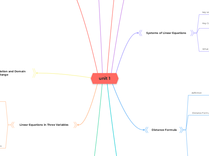
unit 1
Linear Equations in One Variable
Key Phrases !
The sum of a number and 7.
x+7
Seven more than a number.
The difference of a number and 7.
x−7
Seven less than a number.
The product of 2 and a number.
2x
Twice a number.
One-half of a number. 1/2x
The quotient of a number and 7. x/7
Also! when translating sentences into mathematical statements, be sure to read the sentence several times and identify the key words and phrases as well!
key words!
Sum, increased by, more than, plus, added to, total +
Difference, decreased by, subtracted from, less, minus −
Product, multiplied by, of, times, twice ∗
Quotient, divided by, ratio, per /
Is, total, result =
Subtopic
Definition of a Linear Equation in One Variable
A linear equation in one variable is an equation that can be written in the form ax + b = 0, where a and b are real numbers, a≠ 0, and x is the variable
A linear equation is an equation that can be written in the form ax + b = 0 where a and b are real numbers a is not equal to zero
x is a variable
example 2x – 3 = 0 would be a linear equation!
A solution equation is x =
=
3
2
because
=
3
2
is a number that when substituted for x makes the equation a true statement.
The set of all solutions to an equation is called the solution set of the equation.
remember that we can subtract a quantity from both sides of an equation to get an equivalent equation.
To check the answer, we substitute 4 back into the equation. or whichever might of been your answer
Linear Equation:
ax + b = 0
Not a Linear Equation:
2x2+6=0
3 -+4=0
Solving a Linear Equation in One Variable
Simplify both sides of the equation.
Use the distributive property to clear parentheses.
Combine like terms.
• Consider clearing fractions or decimals by multiplying both sides of the equation by the least common denominator (LCD) of all terms.
Use the addition or subtraction property of equality to collect the variable terms on one side of the equation and the constant terms on the other side
Use the multiplication or division property of equality to make the coefficient on the variable term equal to 1
Check the potential solution in the original equation
then Write the solution set.
An equation satisfied by every number that
is a meaningful replacement for the variable
is called an identity.
3(x+ 1) 3x +3
An equation satisfied by some numbers but
not others, such as 2x =4, is called a
conditional equation.
2x= 4
An equation that has no solution, such as
x = x +1, is called a contradiction.
x= x +1
you'd have to decide whether this equation is an identity, a
conditional equation, or a contradiction.
for example when you have an equation such as -2(x+4)+3x=x-8 you would have to 0=0 subtract x and add 8! that would be the solution.
and so when a true statement such as per say the results are 0=0, the equation is an identity, and the solution set is all real numbers.
another way is like this, per say your equation is 5x-4=11, the solutions would be 5x-4=11 if you have that add 4 and you'd get 5x=15, from there divide 5 and you'd get x=3 and so this would be a conditional equation, and its solution set is 3!
Using a Linear Equation in an Application Involving Simple Interest
key words!
Sum: increased by, more than, plus, added to, total (+)
Difference: decreased by, subtracted from, less, minus( -)
Product: multiplied by, of, times, twice ( ⋅)
Quotient: divided by, ratio, per
÷
Equals: is, total, result
=
Interest Applications
In problems involving simple interest, it is often helpful to use the simple interest formula
I=PRT where I is the simple interest earned on a principle investment, p, with an interest rate of r over t
Currency Applications
A new kind of problem we come across in applications is something we call currency problems. These problems involve finding the number of coins or bills given other information about value. It is important to be careful in defining our variables specifically - either for the number of currency or the value of the currency.
Mixing Applications
Mixture problems often include a percentage and some total amount. It is important to make a distinction between these two types of quantities. For example, if a problem states that a 10-ounce container is filled with a 3% saline (salt) solution, then this means that the container is filled with a mixture of salt and water as follows:
Distance Applications
The distance traveled is equal to the average rate times the time traveled at that rate,
d=r.t These problems usually have a lot of data, so it helps to carefully rewrite the pertinent information as you define variables.
Subtopic
Systems of Linear Equations
key words
addition method
an algebraic technique used to solve systems of linear equations in which the equations are added in a way that eliminates one variable, allowing the resulting equation to be solved for the remaining variable; substitution is then used to solve for the first variable
break-even point
the point at which a cost function intersects a revenue function; where profit is zero
consistent system
a system for which there is a single solution to all equations in the system and it is an independent system, or if there are an infinite number of solutions and it is a dependent system
cost function
the function used to calculate the costs of doing business; it usually has two parts, fixed costs and variable costs
inconsistent system
independent system
a system of linear equations with exactly one solution pair
(x.y)
profit function
the profit function is written as
p(x)=r(x)-c(x), revenue minus cost
revenue function
the function that is used to calculate revenue, simply written as R=xp, where x =quantity and p = price
substitution method
an algebraic technique used to solve systems of linear equations in which one of the two equations is solved for one variable and then substituted into the second equation to solve for the second variable
system of linear equations
a set of two or more equations in two or more variables that must be considered simultaneously.
Key Concepts
A system of linear equations consists of two or more equations made up of two or more variables such that all equations in the system are considered simultaneously.
The solution to a system of linear equations in two variables is any ordered pair that satisfies each equation independently.
Systems of equations are classified as independent with one solution, dependent with an infinite number of solutions, or inconsistent with no solution.
One method of solving a system of linear equations in two variables is by graphing. In this method, we graph the equations on the same set of axes
Another method of solving a system of linear equations is by substitution. In this method, we solve for one variable in one equation and substitute the result into the second equation.
A third method of solving a system of linear equations is by addition, in which we can eliminate a variable by adding opposite coefficients of corresponding variables.
It is often necessary to multiply one or both equations by a constant to facilitate elimination of a variable when adding the two equations together.
Either method of solving a system of equations results in a false statement for inconsistent systems because they are made up of parallel lines that never intersect.
The solution to a system of dependent equations will always be true because both equations describe the same line.
Systems of equations can be used to solve real-world problems that involve more than one variable, such as those relating to revenue, cost, and profit.
What are systems of linear equations?
While a linear equation contains just one line, a system of linear equations contains many linear equations. A system of linear equations can contain 2 or more linear equations.
Systems of linear equations in which the lines do not cross
So what does it look like when lines do not intersect? this system takes the form of two parallel lines.
for an example well use this equation, y=-2x+4, y=-2x-4 these are two linear equations
these two lines have an identical slope but a different horizontal displacement. This is what we can expect for all similar systems of linear equations with parallel lines. We also say that this system has "zero solutions" because there are no points at which the two lines intersect.
As previously noted, the most common outcome with systems of linear equations is one in which the two lines cross once and only once.
Here we can see that there are two different linear equations: y=0.5x+2, y=-2x-3
For our lines to be parallel, the two equations need to have very specific characteristics. But for lines to intersect, we can use almost all other values. The chances of the lines not being parallel are much higher. We say that this system of linear equations has "one solution" because the lines intersect once.
The last possibility involves two identical lines that occupy exactly the same coordinates on the plane.
How can two linear equations be different and yet occupy the same coordinates? In this case, we're dealing with two equivalent equations:
y=-2x-4
Although these two equations are different, we can rearrange either one in such a way that it is identical to the second. Therefore, they are equivalent. We say that this type of system has "infinitely many solutions" because the two lines share an infinite number of points.
y+4=-2x
Distance Formula
definition
Distance Formula is a variant of the Pythagorean Theorem that you used back in geometry. The Pythagorean Theorem allows you to relate the three sides of a right triangle; in particular, it allows you to find the length of the third side of a right triangle, given the lengths of the other two sides. The Distance Formula takes two points and implicitly assigns them the role of the hypotenuse.
Distance Formula
Suppose you're given the two points (−2, 1) and (1, 5), and they want you to find out how far apart they are
You can draw in the lines, parallel to the two coordinate axes, that form a right-angled triangle, using these points as two of the corners
to find the lengths of the horizontal and vertical sides of the right triangle: just subtract the x-values and the y-value
Then use the Pythagorean Theorem to find the length of the third side (which is the hypotenuse of the right triangle
the distance formula that will be discussed is based more on the Pythagorean theorem. In a coordinate plane, where the axes are labeled x and y, distance is found by using the formula d = ( x 2 − x 1 ) 2 + ( y 2 − y 1 ) 2 .
key words
hypotenuse
In geometry, a hypotenuse is the longest side of a right-angled triangle, which is the side opposite the right angle. The length of the hypotenuse of a right triangle can be found using the Pythagorean theorem, which states that the square of the length of the hypotenuse equals the sum of the squares of the lengths of the other two sides. For example, if one of the other sides has a length of 3 metres (when squared, 9 m²) and the other has a length of 4 m (when squared, 16 m²), then their square
Delta
Delta is a greek letter that in this case stands for change.
Delta x is the change in x. If the first point (3, 1) and the second point is (1,1), then delta x is the change in x is 3-1 or 2. Delta y is the change in y is 1=1 or 0.
Although it usually refers to change, delta itself is a Greek letter that can also be used as a variable in equations. Typically, if used to signify change, it is followed by another variable, such as ?X.
Deltas are written in both upper and lower case. Upper-case deltas look like triangles (?), and lower-case deltas look like a stylized d (?). When using deltas as the syntax for writing differential equations, the lower-case delta is more common.
Delta is a symbol that means "change" in some quantity.
Writing and Interpreting an Augmented Matrix
what is an Augmented Matrix?
An augmented matrix is a means to solve simple linear equations. The coefficients and constant values of the linear equations are represented as a matrix, referred to as an augmented matrix. In simple terms, the augmented matrix is the combination of two simple matrices along the columns. If there are m columns in the first matrix and n columns in the second matrix, then there would be m + n columns in the augmented matrix.
with the help of three linear equations, represented as follows.
a1x + b1y + c1z = d1
a2x + b2y + c2z = d2
a3x + b3y + c3z = d3
The three above equations can be represented in matrix form with the coefficients as one matrix, the constant terms as another matrix, and the variables as a separate matrix.
The augmented matrix 'M' can be represented as a matrix after combining the matrices with the coefficient terms and the constant terms.
M = [A | B]
An augmented matrix is a matrix that is formed by joining matrices with the same number of rows along the columns. It is used to solve a system of linear equations and to find the inverse of a matrix.
Properties Of Augmented Matrix
The augmented matrix is a rectangular matrix.
The number of columns is equal to the variables in the linear equations and the constant term.
The number of rows is equal to the number of linear equations.
The rows of the augmented matrix can be interchanged.
The elements of a particular row can be multiplied or divided with a constant.
The particular row can be added and subtracted to other rows of the matrix.
The multiple of a row can be added to another row of the matrix.
Finding Inverse of Matrix Using Augmented Matrix
the inverse of the matrix A, we obtain the augmented matrix (A | I), where I is a 3 × 3 identity matrix. We apply elementary row operations on (A | I) to make the left side of the augmented matrix an identity matrix and obtain the matrix (I | A-1).
Important Notes on Augmented Matrix
An augmented matrix is a matrix that is formed by joining matrices with the same number of rows along the columns.
It is used to solve a system of linear equations and to find the inverse of a matrix.
We can apply elementary row operations on the augmented matrix.
The augmented matrix is solved by performing operations across its rows, and it helps to find the solution to the linear equations represented in the augmented matrix. The augmented matrix contains the coefficient values and the constant terms. Applying the Gauss Jordan Method of row transformation, the operations on rows help in transforming a part of the augmented matrix into an identity matrix. The elements remaining in the last column after the row transformations are the values of the variable of the linear equations.
with the notations from the equations of the line. The three equations of the lines are a1x + b1y + c1z = d1, a2x + b2y + c2z = d2, a3x + b3y +c3z = d3. Let us represent these three equations in the form of an augmented matrix.
numerous row operations to obtain the following matrix. We apply elementary row operations to make the left side of the bar an identity matrix and the right side gives the solution to the system of equations.
the elements in the last row represent the values of the variables, and we have x = k, y = l, z = m, respectively.
Applying the Point-Slope Formula
the equation of a straight line in the form y − y1 = m(x − x1) where m is the slope of the line and (x1, y1) are the coordinates of a given point on the line
Subtopic
Point Slope Form
The point slope form is used to find the equation of the straight line which is inclined at a given angle to the x-axis and passes through a given point. The equation of a line is an equation that is satisfied by each and every point on the line. This means that a linear equation in two variables represents a line.
Point slope form is used to represent a straight line using its slope and a point on the line. That means, the equation of a line whose slope is 'm' and which passes through a point (x
1
, y
1
) is found using the point slope form. Different forms can be used to express the equation of a straight line. One of them is point slope form. The equation of the point slope form is:
y - y
1
= m(x - x
1
)
where, (x, y) is a random point on the line and m is the slope of the line
Derivation of Point Slope Formula
how to find the point slope form (i.e. the proof of the formula of the point slope form). We will derive this formula using the equation for the slope of a line. Let us consider a line whose slope is 'm'.
Subtopic
Some of the methods
Point slope form
Slope-intercept form
Intercept form
Two-point form
Linear Equation in Two Variables
Definition
An equation is said to be linear equation in two variables if it is written in the form of ax + by + c=0, where a, b & c are real numbers and the coefficients of x and y, i.e a and b respectively, are not equal to zero.
For example, 10x+4y = 3 and -x+5y = 2 are linear equations in two variables.
The solution for such an equation is a pair of values, one for x and one for y which further makes the two sides of an equation equal.
Solution of Linear Equations in Two Variables
The solution of linear equations in two variables, ax+by = c, is a particular point in the graph, such that when x-coordinate is multiplied by a and y-coordinate is multiplied by b, then the sum of these two values will be equal to c.
Basically, for linear equation in two variables, there are infinitely many solutions.
System of Linear Equations in Two Variables
Instead of finding the solution for a single linear equation in two variables, we can take two sets of linear equations, both having two variables in them and find the solutions. So, basically the system of linear equations is defined when there is more than one linear equation.
For example, a+b = 15 and a-b = 5, are the system of linear equations in two variables. Because, the point a = 10 and b = 5 is the solution for both equation
a+b=10 + 5 = 15
a-b=10-5 = 5
Hence, proved point (10,5) is solution for both a+b=15 and a-b=5.
Subtopic
Example
to find the solution of Linear equation in 2 variables, two equations should be known to us.
5x + 3y = 30
The above equation has two variables namely x and y.
Subtopic
Graphically this equation can be represented by substituting the variables to zero.
The value of x when y=0 is
5x + 3(0) = 30
⇒ x = 6
and the value of y when x = 0 is,
5 (0) + 3y = 30
⇒ y = 10
to solve linear equation in two variables, the two equations have to be known and then the substitution method can be followed
No Solution
If the two linear equations have equal slope value, then the equations will have no solutions.
m1 = m2
Definition of a Relation and Domain and Range
A relation is a set of rules which relates the value of one set to the value of other sets. The domain of a relation is the set of values that we take as input and the range is the set of the values which are obtained in the form of the answers to the relation.
Linear Equations in Three Variables
Solve Systems of Three Equations in Three Variables
In order to solve systems of equations in three variables, known as three-by-three systems, the primary goal is to eliminate one variable at a time to achieve back-substitution. A solution to a system of three equations in three variables
(x,y,z),
is called an ordered triple.
To find a solution
Interchange the order of any two equations.
Multiply both sides of an equation by a nonzero constant.
Add a nonzero multiple of one equation to another equation.
number of possible solutions
Systems that have a single solution are those which, after elimination, result in a solution set consisting of an ordered triple
(x,y,z) Graphically, the ordered triple defines a point that is the intersection of three planes in space.
Systems that have an infinite number of solutions are those which, after elimination, result in an expression that is always true, such as
0=0. Graphically, an infinite number of solutions represents a line or coincident plane that serves as the intersection of three planes in space.
Systems that have no solution are those that, after elimination, result in a statement that is a contradiction, such as 3=0. Graphically, a system with no solution is represented by three planes with no point in common.
Identifying an Inconsistent System Using Reduced Row-Echelon Form
The Elimination Method
solve systems of linear equations algebraically using the elimination method. In other words, we will combine the equations in various ways to try to eliminate as many variables as possible from each equation.
Scaling
we can multiply both sides of an equation by a nonzero number
Swap
we can swap two equations
Replacement
we can add a multiple of one equation to another, replacing the second equation with the result.
Augmented Matrices and Row Operations
the equals sign
=
over and over again, merely as placeholders: all that is changing in the equations is the coefficient numbers. We can make our life easier by extracting only the numbers, and putting them in a box:
This is called an augmented matrix.
The word “augmented” refers to the vertical line, which we draw to remind ourselves where the equals sign belongs; a matrix is a grid of numbers without the vertical line.
Augmented Matrices from Vector Equations
We already saw that systems of linear equations and vector equations are the same thing.
If you have a vector equation, such as the equation in (1.2.1)
then converting it to augmented matrix form is very easy. You can just read off directly that the augmented matrix
that is to say, the columns of the augmented matrix are exactly the column-vectors appearing in the equation. The column of constants in the equation, on the right of the “=” sign, becomes the augmentation column of the matrix.
Row Operations
In augmented matrix notation, our three valid ways of manipulating our equations become row operations
then scaling multiply all entries in a row by a nonzero number.
Here the notation
R1
simply means “the first row”, and likewise for
R2 R3 etc
Replacement
add a multiple of one row to another, replacing the second row with the result.
Swap
nterchange two rows.
olving equations by elimination requires writing the variables x, y .z
Subtopic
A matrix is in reduced row echelon form if it is in row echelon form, and in addition:
Each pivot is equal to 1.
Each pivot is the only nonzero entry in its column
Definition
All zero rows are at the bottom.
The first nonzero entry of a row is to the right of the first nonzero entry of the row above.
Below the first nonzero entry of a row, all entries are zero.
pivot
A pivot is the first nonzero entry of a row of a matrix in row echelon form.
A matrix in row-echelon form is generally easy to solve using back-substitution.